Paper Review : Attention is all you need

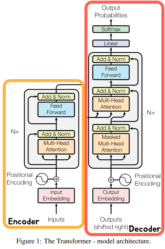
URL: https://arxiv.org/pdf/1706.03762.pdf

저자: Ashish Vaswani,Noam Shazeer,Niki Parmar,Jakob Uszkoreit,Llion Jones,Aidan N. Gomez,Łukasz Kaiser,Illia Polosukhin

1 Background

Limitations of RNN, LSTM model

The structure of RNN involves BPTT (Backpropagation Through Time) for sequentially inputting each element of the sequence data. If the length of sequence increases,

❗ Sequential Computation constraint & Memory constraint problem occurs. <br>

Solving with CNN Model(Extended Neural GPU, ByteNet, ConvS2S)

Parallel processing can handle long sequences, but the number of operations required to relate signals between arbitrary input and output positions increases proportionally with the distance between positions.

❗ difficult to learn dependencies between distant positions

Solving with Transformer

💡 Parallelized computation
💡 Optimized total computation complexity per layer
💡 Able to learn long-range dependencies in the network

2 Model Architecture

1) Attention

Attention

---

Mapping a query and a set of key-value pairs to an output (query, keys, values, ,output are all vectors) output is computed as a weighted sum of the values, where the weight assigned to each value is computed by a compatibility function of the query with the corresponding key.

💡  output = sum( w X value)

                        w =  query & key compability 

• What is query, key ,value and output?

  Input sentence (English): “I love cats”

  Output sentence (Korean): “나는 고양이를 사랑해”

  Imagine we are at the point of generating the word “사랑해” in Korean, which corresponds to “love” in English.

  • Query (Q): This would represent our current focus, the word “love”.
  • Keys (K): For simplicity, let’s assume the keys are representations of each word in the English sentence - [“I”, “love”, “cats”].
  • Values (V): These are also representations of each word in the English sentence. However, whereas keys are like “labels” to help access the information, values contain the actual details.
  • Output: The final output, after the attention mechanism, is a representation heavily influenced by “love” and, to a lesser extent, “I”. This will help the model decide that the most appropriate translation at this point is “사랑해”.

How do you calculate query & key compability?

Two most commonly used attention functions are Additive Attention & Dot product Attention.

Additive Attention

• Attention Score=vT⋅tanh(W1⋅Q+W2⋅K)
• v, W1,W2 learning parameter
• Additive attention computes the compatibility function using a feed-forward network with a single hidden layer.

• more info

  Additive Attention은 주로 Bahdanau attention이라고도 불리며, 이는 2015년에 Dzmitry Bahdanau와 그의 동료들에 의해 소개되었습니다. 이 attention 메커니즘은 encoder-decoder 구조에서 주로 사용되며, decoder의 각 단계에서 encoder의 모든 단계와의 alignment를 학습합니다.

  Additive attention의 핵심 아이디어는 query(주로 decoder의 현재 상태)와 key(주로 encoder의 모든 상태)를 함께 사용하여 attention score를 계산하는 것입니다. 이 attention score는 이후에 value(주로 encoder의 상태)에 가중치를 부여하여 weighted sum을 생성하는데 사용됩니다. 이러한 방식으로, decoder는 encoder의 모든 상태에 대한 다양한 중요도를 학습할 수 있게 됩니다.

  Additive attention의 수식은 다음과 같습니다:

  이 수식은 먼저 query와 key 벡터를 연결하고, 이 연결된 벡터에 가중치 행렬 Wa를 적용한 다음, tanh 활성화 함수를 통과시킵니다. 결과적으로 얻어진 벡터에 다른 가중치 벡터 va를 적용하여 최종 attention score를 얻습니다. 이 score는 이후에 softmax 함수를 통과하여 attention 가중치를 생성하고, 이 가중치는 value 벡터의 가중합을 계산하는데 사용됩니다.

Dot Product Attention

https://wikidocs.net/86900

• Attention Score=Q⋅KT
• Dot-product attention is much faster and more space-efficient in practice, since it can be implemented using highly optimized matrix multiplication code.

Attention used in Transformer : Scaled Dot Product Attention

queries and keys of dimension dk, and values of dimension dv Scaled : 1/√dk solving gradient vanishing problem

the dot products grow large in magnitude, pushing the softmax function into regions where it has extremely small gradients . To counteract this effect, we scale the dot products 1/√dk

→ For example, imagine two large vectors. The dot-product between them is the sum of the products of each element, so if the dimension of the vectors is large, this value can become very large.This results in the input to the softmax function becoming very large, consequently, the resulting probability distribution becomes very ‘sharp’.

In other words, the probability at one position becomes close to 1, and the probabilities at all other positions become close to 0. The gradient of such a probability distribution becomes very small, which increases the likelihood of gradient vanishing during back propagation.

• Large values of dk, additive attention outperforms dot product attention without scaling for larger values of dk.

• Small values of dk, the two mechanisms perform similarly.

  💡 Optimized total computation complexity per layer

Attention used in Transformer: Multi-Head Attention

Instead of performing a single attention function with keys, values and queries, we found it beneficial to linearly project the queries, keys and values with different, learned linear projections h times.

💡 Flexibility 
able to pay attention to different words in the input sequence

💡 Richer Representation 
multiple heads can learn a different aspect of the relationship between the words in the sequence

• single head - dmodel(embedding dimension)

  

• Multi head - h different heads , every head with dk dimension

  In this work we employ h = 8 parallel attention layers, or heads. For each of these we use dk = dv = dmodel/h = 64. Due to the reduced dimension of each head, the total computational cost is similar to that of single-head attention with full dimensionality.

Given a 4-dimensional embedding vector for the word “love” and with 2 attention heads, we multiply the vector by a 4x2 weight matrix to generate 2-dimensional (4/2) query, key, and value representations for each head

💡 Parallelized computation : each head, each attention

💡 Optimized total computation complexity per layer

2) Positional Encoding

Transformer contains no recurrence and no convolution, in order for the model to make use of the order of the sequence, we must inject some information about the relative or absolute position of the tokens in the sequence.

pos is the position and i is the dimension

https://www.youtube.com/watch?v=zxQyTK8quyY&t=644s

We also experimented with using learned positional embeddings instead, and found that the two versions produced nearly identical results. We chose the sinusoidal version because it may allow the model to extrapolate to sequence lengths longer than the ones encountered during training.

3) Position-wise Feed-Forward Networks

Two linear transformations with a ReLU activation and two different parameters.

Enables model to learn more complex pattern.

4) Transformer

3 types of attention

What is Self-attention ?

---

In self-attention Q,K, V comes from same vector.

Q :Every token vectors of input sentence K : Every token vectors of input sentence V : Every token vectors of input sentence

the model is applying attention to its own input to compute a representation of the sequence

1 Encoder self-attention

---

The encoder contains self-attention layers.

In a self-attention layer all of the keys, values and queries come from the same place, in this case, the output of the previous layer in the encoder. Each position in the encoder can attend to all positions in the previous layer of the encoder.

2 Masked Decoder self-attention

---

Self-attention layers in the decoder allow each position in the decoder to attend to all positions in the decoder up to and including that position. We need to prevent leftward information flow in the decoder to preserve the auto-regressive property. We implement this inside of scaled dot-product attention by masking out (setting to −∞) all values in the input of the softmax which correspond to illegal connections.

3 Encoder-Decoder attention

---

The queries come from the previous decoder layer and the memory keys and values come from the output of the encoder. This allows every position in the decoder to attend over all positions in the input sequence.

Encoder

Decoder

3 Why Self-attention

1) Complexity per Layer

Self-Attention:

The core operation of the Self-Attention mechanism is a matrix multiplication, specifically the dot product between the Query and Key matrices.

Assuming a sequence length of n, both the Query and Key are of size n X d. The complexity for this matrix multiplication operation is O(n^2 X d). Additionally, there’s another operation to multiply with the Value matrix to compute the output, so the overall complexity remains O(n^2 X d).

RNN (Recurrent Neural Networks):

The core operation of RNNs involves matrix multiplication for the current input and the previous hidden state. Assuming a hidden state dimension of d, this operation has a complexity of O(d^2). Since this operation is carried out for each step in the sequence, the overall complexity for the entire sequence is O(n X d^2), where n is the length of the sequence.

• more explanation

  RNN은 각 시간 스텝마다 이전 시간 스텝의 hidden state와 현재 시간 스텝의 입력을 가져와 새로운 hidden state를 계산합니다.

  RNN의 핵심 업데이트 연산

  여기서:

  • h_t는 시간 t 에서의 hidden state입니다.
  • h_t-1는 이전 시간 스텝의 hidden state입니다.
  • x_t 는 시간 t 에서의 입력입니다.
  • W_hh와 W_xh 는 학습 가능한 가중치 행렬이며, b 는 바이어스 벡터입니다.
    1. Matrix-Vector Multiplication: W_hh h_t-1 의 연산 복잡도는 O(d^2) 입니다. 왜냐하면 W_hh 는 d X d 행렬이고, h_t-1 는 d차원 벡터이기 때문입니다.
    2. Sequence Length: RNN은 시퀀스의 각 요소를 차례대로 처리하므로, 연산은 시퀀스의 길이 n 에 선형적으로 비례합니다. 따라서 각 시간 스텝에서의 복잡도는 O(d^2)이며, 전체 시퀀스를 위한 복잡도는 O(n d^2)입니다.
       

CNN (Convolutional Neural Networks):

The complexity of a 1D convolution operation depends on the length of the input n, the length of the kernel k, and the dimension of both input and output d. For each position in the input, a matrix multiplication with dimension k has to be performed. Thus, the computational complexity for one input position is O(k X d^2). For the entire input, the complexity is O(k X nX d^2).

2) Sequential Operations

Self-attention layer connects all positions with a constant number of sequentially executed operations, whereas a recurrent layer requires O(n) sequential operations.

3) Maximum Path Length

The shorter paths between any combination of positions in the input and output sequences, the easier it is to learn long-range dependencies.

• more explanation

  CNNs inherently have a hierarchical structure. When we apply a convolution with a kernel of size k to an input, we are essentially creating a local window or receptive field of size k over the input. Each successive layer in a deep CNN expands this receptive field.

  The reason the maximum path length in CNNs can be characterized as O(log_k(n)) lies in how these receptive fields expand as we go deeper into the network:

  1. First Layer: The receptive field is k (the size of the kernel).
  2. Second Layer: The receptive field becomes k + (k-1) , because each unit in the second layer can “see” k units from the first layer, and each of those can see k original input units. But note that there’s an overlap of k-1 between adjacent receptive fields from the first layer.
  3. Third Layer: The receptive field further grows, taking into account the expanded field of the second layer.

  Given a large enough depth and assuming stride of 1 and no pooling (or pooling with window size 1 and stride 1), a CNN can cover or “see” the entire input.

  The depth required to cover a sequence of length n with a kernel of size k is logarithmic in n with a base k, hence the O(log_k(n)) ) notation. The intuition is that with each subsequent layer, the receptive field grows by a factor determined by the kernel size, and the number of layers required to cover an input of size n grows logarithmically with respect to n.

RNN vs Self-Attention

---

In terms of computational complexity, self-attention layers are faster than recurrent layers when the sequence length n is smaller than the representation dimensionality d, which is most often the case with sentence representations used by state-of-the-art models in machine translations, such as word-piece and byte-pair representations. To improve computational performance for tasks involving very long sequences, self-attention could be restricted to considering only a neighborhood of size r in the input sequence centered around the respective output position. This would increase the maximum path length to O(n/r).

• more explanation

  The statement suggests a modification to the standard self-attention mechanism to make it more computationally efficient for very long sequences. By default, in self-attention, every token in the sequence can attend to every other token, which means the “path” between any two tokens is direct and short.

  However, if we restrict self-attention to only consider a neighborhood of size r around each token, then tokens outside of this neighborhood can’t be “seen” directly. If a token wants to gather information from another token outside its immediate neighborhood, it now has to rely on a chain of intermediate tokens and potentially additional layers in the network to bridge the gap.

  The concept of “path length” here refers to the number of steps or layers it takes for information to travel between distant tokens. In the modified attention mechanism, the path length increases because, instead of every token attending to every other token directly, now tokens can only attend to those within their immediate neighborhood of size r. Therefore, to get information from tokens that are further away, the information needs to “hop” across multiple neighborhoods, increasing the path length.

  The notation O(n/r) captures this increase in path length. As r(the neighborhood size) decreases, the number of these “hops” or intermediate steps, and thus the path length, increases. Conversely, if r is large, meaning the neighborhood is broad, the path length would be shorter.

4 Training

Base Model:

• Hidden units of feed-forward network: 2048
• Model dimension (d_model): 512
• Self-attention heads: 8
• Number of encoder & decoder stacks: 6 each

Big Model:

• Hidden units of feed-forward network: 8192
• Model dimension (d_model): 1024
• Self-attention heads: 16
• Number of encoder & decoder stacks: 6 each

1) Training Data and Batching

WMT 2014 English-German dataset

4.5 million sentence pairs, 37000 tokens

WMT 2014 English-French dataset

36M sentences ,split tokens into a 32000 word-piece vocabulary

Each training batch contained a set of sentence pairs containing approximately 25000 source tokens and 25000 target tokens.

• token/ word-piece vocabulary
  1. Token: A token is a unit of text that a document is split into for the purpose of analysis or processing, primarily in the field of Natural Language Processing (NLP). Tokens can be as short as a single character or as long as a word. For instance, the phrase “ChatGPT is great!” can be tokenized into [“ChatGPT”, “is”, “great”, “!”].
  2. Word Piece Vocabulary (or subword tokenization): Word pieces are a way of splitting words into smaller, more manageable pieces. Instead of splitting by words, a tokenizer that employs word piece vocabulary might split words into subwords or characters, especially for languages with compounding or agglutination, or to handle out-of-vocabulary words. For example, the word “unhappiness” could be split into subword tokens like [“un”, “happiness”] or even [“un”, “happi”, “ness”]. Word piece vocabulary is particularly useful for languages where word boundaries are not as clear as spaces in English.

  Difference: While both tokens and word pieces are units of text, the main distinction lies in their granularity and usage. Tokens typically represent larger chunks like words or punctuation, while word pieces can represent smaller units within words, allowing for more flexibility in tokenizing especially when handling less common words or morphemes.

• source token / target token
  1. Source Token: A source token is an individual unit (like a word or subword) from the sentence in the source language. In machine translation, the model takes in these source tokens to generate corresponding tokens in the target language. For instance, in translating from English to French, English words or subwords are the source tokens.
  2. Target Tokens: Target tokens are the individual units (like words or subwords) in the target language that the model aims to produce as output. Continuing with the English to French translation example, the French words or subwords that the model generates would be the target tokens.

2) Hardward and Schedule

• 8 NVIDIA P100 GPUs
• trained the base models for a total of 100,000 steps or 12 hours.
• trained big models 300,000 steps or 3.5 days

3) optimizer

• Adam optimizer with β1 = 0.9, β2 = 0.98 and ϵ = 10−9.
• Varied the learning rate over the course of training, according to the formula:

warmup_steps = 4000.

This corresponds to increasing the learning rate linearly for the first warmup_steps training steps, and decreasing it thereafter proportionally to the inverse square root of the step number .

4) Regularization

• Residual Dropout

  Applied dropout to the output of each sub-layer, before it is added to the sub-layer input and normalized. In addition, we apply dropout to the sums of the embeddings and the positional encodings in both the encoder and decoder stacks. For the base model, we use a rate of Pdrop = 0.1.

• Label Smoothing

  During training, employed label smoothing of value ϵls = 0.1 .

  This hurts perplexity, as the model learns to be more unsure, but improves accuracy and BLEU score.

  • Label Smoothing

    Cross Entropy Loss function

    

    Label Smoothing Loss funtion

    

    In deep learning, especially in classification tasks, it’s common for the model to predict the probability of a particular class as 1 (or very close to 1) and all other classes as 0 (or very close to 0). While this may seem like a desired behavior, it can actually cause some issues:

    1. Overconfidence: The model becomes overly certain about its predictions, which might not be ideal, especially if the model’s prediction is incorrect.
    2. Poor Generalization: Such overconfident behavior can lead to reduced generalization capabilities, particularly when the model encounters previously unseen data.

    Label smoothing is a regularization technique that addresses this issue. It works by slightly adjusting the target distribution for each label. Instead of using a “hard” one-hot encoded vector where the correct class is 1 and all others are 0, the labels are “smoothed” by assigning a small value to the non-target labels.

    For example, for a three-class classification problem, the true label [1, 0, 0] might be smoothed to something like [0.9, 0.05, 0.05] when using label smoothing.

    The benefits of label smoothing include:

    1. Preventing Overconfidence: By ensuring the model never sees the absolute certainty in the training dataset, it’s less likely to produce overly confident predictions.
    2. Improved Generalization: Label smoothing can provide better generalization on the test set and lead to more calibrated probability estimates.
    3. Stability: It can stabilize the training process because it prevents the log likelihood from blowing up in case of wrong predictions.

    However, it’s worth noting that the choice of the smoothing parameter requires some experimentation, as too much smoothing might dilute the signal from the labels, while too little might not have the desired effect.

    https://hongl.tistory.com/230

  • Perplexity

    Perplexity is one of the metrics to evaluate the performance of a language model. Specifically, it measures the probability of the language model for a given data set. Perplexity is defined as:

    Where b is the base (usually 2 or e ), N is the total number of tokens, and p(w_i) is the probability of the i-th word.

    A lower Perplexity value indicates that the language model is performing better on the test data. In other words, it means the probability distribution predicted by the model is closer to the actual probability distribution of the data.

5 Results

1) Machine Translation

• BLEU (Bilingual Evaluation Understudy)
  • Purpose: BLEU is a metric for evaluating the quality of machine-translated text. It measures how many n-grams (sequences of n words) in the machine-translated text match the n-grams in the reference text.
  • Calculation: The score is calculated based on precision for each n-gram (unigrams, bigrams, trigrams, etc.), and then these precision scores are combined into a single score. It also incorporates a penalty for translations that are shorter than the reference, called the “brevity penalty.”
  • Value Range: The score ranges from 0 to 1, with 1 indicating a perfect match with the reference translation. Typically, the score is multiplied by 100 to get a percentage.
  • Limitation: While BLEU is widely used, it has limitations. For instance, a high BLEU score doesn’t always correlate with human judgment of translation quality, especially for sentences taken out of context.
• FLOPS(Floating Point Operations Per Second)
  1. Definition: FLOPS is a metric used to measure the performance of a computer. It represents the number of floating-point operations a processor or system can perform in one second.
  2. Floating-Point Operations: These operations refer to computations involving real numbers and are crucial in various fields such as science, engineering, graphics, and deep learning. They can be more complex and time-consuming compared to integer operations.
  3. Calculating FLOPS: It measures the total number of floating-point operations executed in a given period to derive the FLOPS value. For instance, 1 TFLOPS indicates that up to one trillion operations can be executed in one second.
  4. FLOPS in Deep Learning: With the increasing size and complexity of deep learning models, FLOPS has become an essential metric to evaluate the computational requirements of a model. Large models, in particular, have many operations to perform, leading to a significant increase in FLOPS. Networks like BERT or GPT, for example, might require tens to hundreds of trillions of operations to process a single input.
  5. Caveat: FLOPS solely measures computational capacity. Therefore, a system with high FLOPS doesn’t always guarantee superior real-world performance. Other factors like memory bandwidth and I/O can become performance bottlenecks.

  

• The Transformer (big) model trained for English-to-French used dropout rate Pdrop = 0.1, instead of 0.3.

• We used beam search with a beam size of 4 and length penalty α = 0.6. These hyperparameters were chosen after experimentation on the development set. We set the maximum output length during inference to input length + 50, but terminate early when possible.

  Beam Search with a beam size of 4:

  • Beam search is a heuristic search algorithm used in machine learning, especially in sequence-to-sequence models. Its primary objective is to find the most probable sequence of tokens (e.g., words) that can be produced as an output.
  • The term beam size refers to the number of sequences that are considered at any given time during the search process. A beam size of 4 means that the algorithm keeps track of the top 4 most probable sequences at each step.

  Length penalty α = 0.6:

  • This indicates that there’s a penalty applied based on the length of the generated sequence. The length penalty helps in controlling the length of the output sequences.
  • An α value less than 1 tends to favor shorter sequences, whereas an α greater than 1 would favor longer sequences. In this context, an α of 0.6 means the model might have a slight bias towards producing shorter sequences.

• The number of floating point operations used to train a model estimation

  training time X the number of GPUs used X sustained single-precision floating-point capacity

  • sustained single-precision floating-point capacity
    1. Single-Precision Floating-Point: This refers to a method of encoding real numbers in a way that they can be used in floating-point arithmetic. In many computer systems, single-precision floating-point numbers are represented using 32 bits, following the IEEE 754 standard for floating-point arithmetic. This format can represent a wide range of values with varying levels of precision, suitable for many computational tasks.
    2. Capacity: In the context of computing performance, capacity typically refers to the maximum potential or capability of a system to execute tasks.
    3. Sustained: This adjective is crucial. While any system might peak at a certain number of operations per second, it’s not always able to maintain (or “sustain”) this level of performance for extended periods. “Sustained” refers to the long-term, consistent performance level a system can achieve, rather than its short-term peak.

    Combining these terms, “sustained single-precision floating-point capacity” refers to the long-term and consistent computational capability of a system when dealing with single-precision floating-point arithmetic. It provides a more realistic measure of a system’s performance in practical scenarios involving floating-point calculations, as opposed to its theoretical peak capacity.

2) Model Variations

• rows (A), we vary the number of attention heads and the attention key and value dimensions,keeping the amount of computation constant. While single-head attention is 0.9 BLEU worse than the best setting, quality also drops off with too many heads.
• rows (B), we observe that reducing the attention key size dk hurts model quality. This suggests that determining compatibility is not easy and that a more sophisticated compatibility function than dot product may be beneficial.
• rows (C) and (D) that, as expected,bigger models are better, and dropout is very helpful in avoiding over-fitting.
• row (E) we replace our sinusoidal positional encoding with learned positional embeddings, and observe nearly identical results to the base model.

3) English Constituency Parsing

• English constituency parsing

  English constituency parsing, often just referred to as constituency parsing, is a natural language processing task that involves analyzing and breaking down a sentence into its constituent parts (or constituents) and representing them hierarchically in a tree structure. This tree structure, commonly called a “parse tree” or “syntax tree”, showcases the syntactic structure of a sentence according to a given grammar.

  In a parse tree:

  • The leaves (or terminal nodes) are the words of the sentence.
  • The internal nodes represent linguistic constituents (e.g., noun phrases, verb phrases, etc.).
  • The edges (or branches) indicate dominance relations between the constituents.

  For example, consider the sentence “The cat sat on the mat.” A simplistic parse tree might break this sentence down into a noun phrase (“The cat”) and a verb phrase (“sat on the mat”), with further breakdowns within each of those phrases.

  The primary purpose of constituency parsing is to uncover the syntactic structure of a sentence, which can be crucial for many downstream applications like machine translation, question answering, and sentiment analysis. Different from dependency parsing, which represents grammatical relations between words, constituency parsing captures how words group together to form larger units within a sentence.

challenges Output is subject to strong structural constraints and is significantly longer than the input. RNN sequence-to-sequence models have not been able to attain state-of-the-art results in small-data regimes.

Training

• 4-layer transformer
• dmodel = 1024
• Performed only a small number of experiments to select the dropout, both attention and residual, learning rates and beam size on the Section 22 development set, all other parameters remained unchanged from the English-to-German base translation model.

WSJ only

• Wall Street Journal (WSJ) portion of the Penn Treebank, about 40K training sentences.
• vocabulary of 16K tokens

semi-supervised setting

• using the larger high-confidence
• BerkleyParser corpora from with approximately 17M sentences.
• vocabulary of 32K tokens

Inference

• increased the maximum output length to input length + 300.
• used a beam size of 21 and α = 0.3 for both WSJ only and the semi-supervised setting.

Result

Despite the lack of task-specific tuning our model performs surprisingly well, yielding better results than all previously reported models with the exception of the Recurrent Neural Network Grammar . In contrast to RNN sequence-to-sequence models, the Transformer outperforms the BerkeleyParser.

6 Conclusion

In this work, we presented the Transformer, the first sequence transduction model based entirely on attention, replacing the recurrent layers most commonly used in encoder-decoder architectures with multi-headed self-attention. For translation tasks, the Transformer can be trained significantly faster than architectures based on recurrent or convolutional layers. On both WMT 2014 English-to-German and WMT 2014 English-to-French translation tasks, we achieve a new state of the art. In the former task our best model outperforms even all previously reported ensembles. We are excited about the future of attention-based models and plan to apply them to other tasks. We plan to extend the Transformer to problems involving input and output modalities other than text and to investigate local, restricted attention mechanisms to efficiently handle large inputs and outputs such as images, audio and video. Making generation less sequential is another research goals of ours.